Learning From Partially Observed Data
Table of contents
Hidden Variables and Missing Data
Missing Data: In practice data entries are often missing resulting in incomplete information to specify a likelihood.
Latent Variables: Latent or hidden variables are variables that are essential for the model description but never observed. For instance, the topic of a document, the category of a user, …
Non-latent Variables: The non-latent variables may be split into observed (those for which we actually know the state) and unobserved (missing) (those whose states would nominally be known but are missing for a particular datapoint).
Augmented Data: Missingness variables are introduced, they indicate whether the variable is observed or not.
Missing Completely at Random (MCAR)
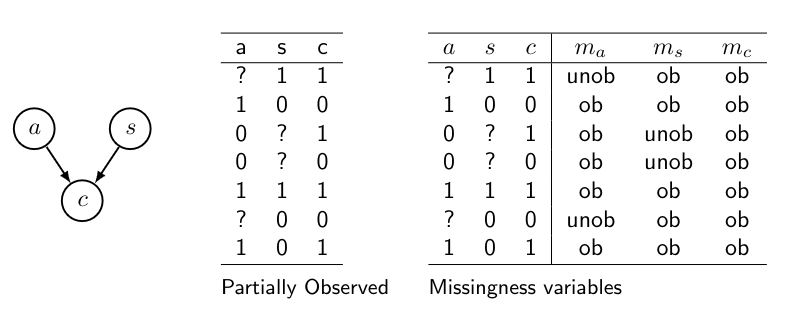
Lets say we have the following BN with missing data:

\(c\) is always observed, so \(m_c\) is deterministic, so it can be left out. (\(m_x\) only indicated whether \(x\) is observed or not)
MCAR assumes that the variables \(x\) in the BN, and the missingness variables \(m\), are independent, that is \(x \perp\!\!\!\perp m\).
Suppose we want to learn the parameters for the conditional probability \(p(x \mid y)\). Under MCAR assumption, we have that \(x, y \perp\!\!\!\perp m\), which means that:
\[\begin{align} p(x,y,m) &= p(x,y) p(m) \\ p(x,y, m=ob) &= p(x,y) p(m=ob) \\ p(x,y) &= p(x,y \mid m=ob) \\ p(x \mid y) &= p(x \mid y, m=ob) \end{align}\]Therefore, the probability \(p(x \mid y)\) can be estimated from \(p(x \mid y, m=ob)\). We know how to do this: it is the probability \(p(x\mid y)\) for the cases where everything is fully observed \((m=ob)\).
How can we calculate that \(\theta_s = p(s=1)\)?
We have two cases:
Complete case-analysis:
| a | s | c | \(m_a\) | \(m_s\) |
|---|---|---|---|---|
| 1 | 0 | 0 | ob | ob |
| 1 | 1 | 1 | ob | ob |
| 1 | 0 | 1 | ob | ob |
Here we use listwise deletion (m = ob), so we only use the complete data entries.
Listwise deletion estimates only from complete data entries (m = ob):
\[p(s) = p(s \mid m_a = ob, m_s = ob) \approx 1/3\]Available case-analysis:
| a | s | c | \(m_a\) | \(m_s\) |
|---|---|---|---|---|
| ? | 1 | 1 | unob | ob |
| 1 | 0 | 0 | ob | ob |
| 1 | 1 | 1 | ob | ob |
| ? | 0 | 1 | unob | ob |
| 1 | 0 | 1 | ob | ob |
Here we use \(p(s)\) pairwise deletion (\(m_s = ob\)), so we only use the entries where \(m_s\) is observed.
Pairwise deletion also learns from data where only non-relevant variables are missing:
\[p(s) = p(s \mid m_s = ob) \approx 2/5\]Both methods will give good estimates if enough data is available, provided that the missing data are MCAR.
Missing at Random (MAR)
The MCAR assumption is stong and does not often hold in real-world data. It is more common to assume that the data is missing at random (MAR). This assumption holds if the missingness variables are conditionally independent of the partially-observed variables \(x_m\) given the fully-observed variables \(x_o\), i.e, if \(x_m \perp\!\!\!\perp m \mid x_o\). Graphically, this corresponds to a missingness graph where the m are allowed to have parents that are fully observed:

This represents e.g. that people diagnosed with cancer (c=1) are more likely to hide private information, i.e. more likely not to tell doctors whether they smoked or not. (p(m=ob) is lower)
Deletion methods (MCAR) lead to biased parameter estimates on MAR data. Suppose we are interested in learning the parameter for \(p(c=1 \mid a = 0, s=1)\) whose true value is 0.3. Listwise or pairwise deletion (they are identical in this case) would in the end estimate the parameter as:
\[\begin{align}p(c=1 \mid a=0, s=1, m=ob) &= p(c=1 \mid a=0, s=1, m_a=ob, m_s=ob) \\ &= p(c=1 \mid a=0, s=1, m_s=ob) \\ &= \frac{p(c=1, m_s=ob \mid a=0, s=1)}{p(m_s = ob \mid a=0, s=1)} \\ &= \frac{p(c=1 \mid a=0, s=1)p(m_s=ob \mid c=1)}{\sum_c p(c \mid a=0, s=1)p(m_s=ob \mid c)} \\ &= \frac{0.3 \times 0.2}{0.3 \times 0.2 + 0.7 \times 0.9} = 0.087 \end{align}\]Missing Not at Random (MNAR)
MNAR missingness mechanisms are in general non-identifiable. This means that there exists no two different BNs and missingness mechanisms that generate the same data. The distribution over the observed values is identical.
Maximum Likelihood with Missing Data
The likelihood for complete data is:
\[L(\theta \mid D) = p(D \mid \theta) = \prod_{i=1}^N p(d_i \mid \theta)\]Where \(N\) is the dataset size and \(d_i\) represents the assignments made in the \(i\)th complete example of the dataset.
For the Marginal Likelihood for partially observed data we have:
\[L(\theta \mid D) = p(D \mid \theta) = \prod_{i=1}^N p(d_i \mid \theta) = \prod_{i=1}^N \sum_{h_i} p(d_i, h_i \mid \theta)\]with \(h_i\), the hidden variables in example \(i\).
Expectation Maximization (EM)
EM is an iterative algorithm that produces a sequence of parameters estimates \(\theta^0, \theta^1, \theta^2, \dots\).
the initial parameters \(\theta^0\) are set arbitrarily. Next, EM iteratively performs two steps:
- Complete the missing data using parameters \(\theta^{i-1}\)
- Estimate new parameters \(\theta^i\) on the completed data.
These steps are repeated until either \(\theta^i\), or the marginal likelihood \(L(\theta^i \mid D)\) have converged.
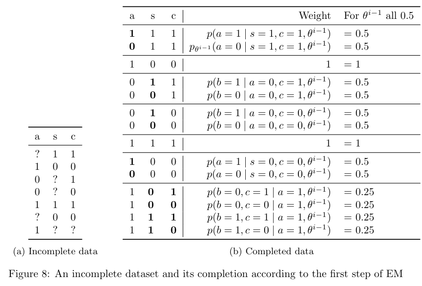
The first step of EM is shown below. The completed data set contains all possible ways of filling in the missing values in the incomplete data. Every complete data case gets assigned a weight, which is the probability of that completion according to the parameters \(\theta^{i-1}\). For example, completing the case \((?, 1,1)\) to \((1,1,1)\) has weight \(p_{\theta^{i-1}} (a=1 \mid s=1, c=1)\).

Computing these weights requires running inference in the BN with parameters \(\theta^{i-1}\). Note that the weights for all the complete cases that come from the same incomplete case sum to one. The last column shows the weights when \(\theta^{i-1}\) sets all parameters in the network to 0.5.
The second step of EM estimates new parameters \(\theta^i\) from the completed data. When dealing with standard complete data, we estimate the parameter \(\theta_{x \mid y}\) as \(\prod_D(xy)/ \prod_D(y)\), where \(\prod_D(z)\) is the number of cases in \(D\) where \(z\) is true. However, in the EM algorithm, our complete-data cases have weights. We can define the expected count \(\prod_{D,i-1}(z)\) as the sum of weights of all complete cases where \(z\) holds, according to the parameters \(\theta^{i-1}\). The figure below shows the expected counts for completed data in the figure above. From these expected counts, we estimate the new parameter \(\theta^i_{x \mid y}\) as \(\prod_{D,i-1}(xy)/\prod_{D,i-1}(y)\).

Suppose that we have seeded \(\theta^0\) such that all parameters are 0.5. The last column of the figure above shows the expected counts under \(\theta^0\) for every complete data case. In the first iteration of EM, we estimate the parameters \(\theta^1\) from this table. For example, \(\theta_{a=1}^1 = (1.75+ 0.25 + 0.25 + 1.75)/7 = 4/7\) and \(\theta_{c=1 \mid a=0,s=0}^1 = (0.5)/(1+0.5) = 1/3\). Thus, in the first iteration of EM, the parameter \(\theta_{a=1}\) increases, and the parameter \(\theta_{c=1 \mid a=0,s=0}\) decreases. These new parameters will induce new weights for the completed data in the next iteration. In turn, this will change the expected counts and lead to new parameter estimates.