Ray Tracing

---

Table of contents

1. How does it work?
2. Ray
   1. Ray-Sphere Intersection
   2. Ray-Triangle Intersection
3. Camera Coordinate System
   1. Viewing coordinates
4. Viewing Rays
5. Intersecting Transformed Objects
6. Simple Stochastic Ray Tracing
   1. How do we stop the recursion? (Russian Roulette)

How does it work?

1. Cast a ray from the camera through each pixel in the image plane.
2. Find the closest object that intersects the ray.
3. Compute the color of the object at the intersection point.
4. Repeat for each pixel.

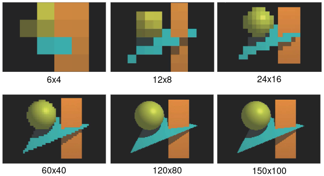
The size of the view plane will determine the quality of the image. The larger the view plane, the better the quality of the image.

Ray

A ray is an infinite straight line that starts at a point o, called the origin, and extends infinitely in some direction d. It is parametrized with the ray parameter t, where \(t=0\) at the ray origin, so that an arbitrary points p on a ray can be expressed as:

\[p(t) = o + td\]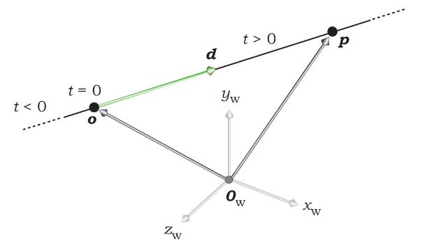

Ray-Sphere Intersection

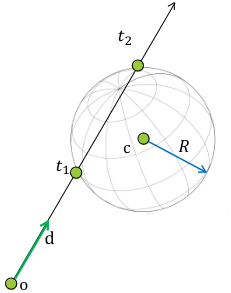
A sphere is defined by its center c and its radius R. Where \(\| p(t) - c\|^2 = R^2\). If we substitute the ray equation into the sphere equation, we get a quadratic equation in \(t\):

\[(p(t) - c) \cdot (p(t) - c) - R^2 = 0\] \[(o + td - c) \cdot (o + td - c) - R^2 = 0\] \[(d \cdot d)t^2 + 2d \cdot (o - c)t + (o - c) \cdot (o - c) - R^2 = 0\]

This will have 0, 1 or 2 solutions. We want the smallest t-value > 0. (t-values < 0 will be behind the observer)

Ray-Triangle Intersection

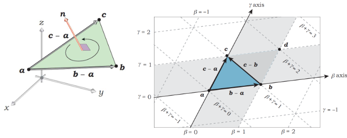
Given 3 points a, b, c, eacht point p in the plane (a, b, c) can be expressed as:

\[p = a + \beta(b - a) + \gamma(c - a)\] \[p = (1 - \beta - \gamma)a + \beta b + \gamma c\] \[p = \alpha a + \beta b + \gamma c \text{, where } \alpha = 1 - \beta - \gamma\]

where \(\beta\) and \(\gamma\) are the barycentric coordinates of the point p.

p is inside the traingle formed by a, b, c, if \(0 < \alpha, \beta, \gamma < 1\).

Camera Coordinate System

How do we define the coordinate system of the camera?

Viewing coordinates

First we need to define a viewing direction l. We then define a vector w which is defined as:

\[w = \frac{(e-l)}{\|e-l\|}\]

Where e is the position of the camera.

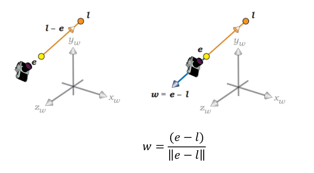
We then define a vector u which is defined by using a up vector which is perpencidular to l. We then get u by:

\[u = \frac{up \times w}{\|up \times w\|}\]

When we have w and u, we can define v by:

\[v = w \times u\]

Which makes sure that w, u and v are all perpendicular to each other.

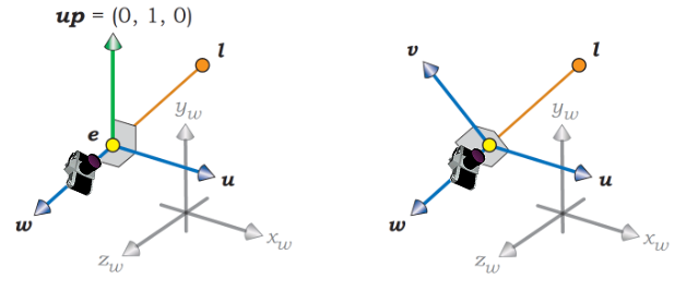
Viewing Rays

How do we define the viewing rays?

We have an origin e and a direction d which is defined as:

\[d = x \cdot u + y \cdot v - d \cdot w\]

Where x, y and z are scalars.

x and y are defined by the pixel coordinates on the image plane.

\[x = s(c - h_{\text{res}}/2 + 0.5)\] \[y = s(c - v_{\text{res}}/2 + 0.5)\]

where c and r are the column and row coordinate respectively. s is the size of a pixel in the image plane. These equations make sure that the point (0,0) is in the center of the image plane. Instead of in one of the corners.

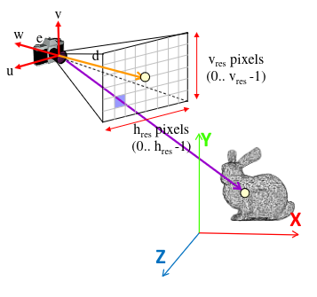
So far we shoot a single ray trough the center of each pixel. But what happends when we have mixed conetent? One solution is using the color that is at the center of the pixel. But this will give a phenomenon called aliasing.

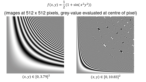
As you can see in the image above we get a lot of aliasing artifacts. We can solve this by using anti-alising.

Intersecting Transformed Objects

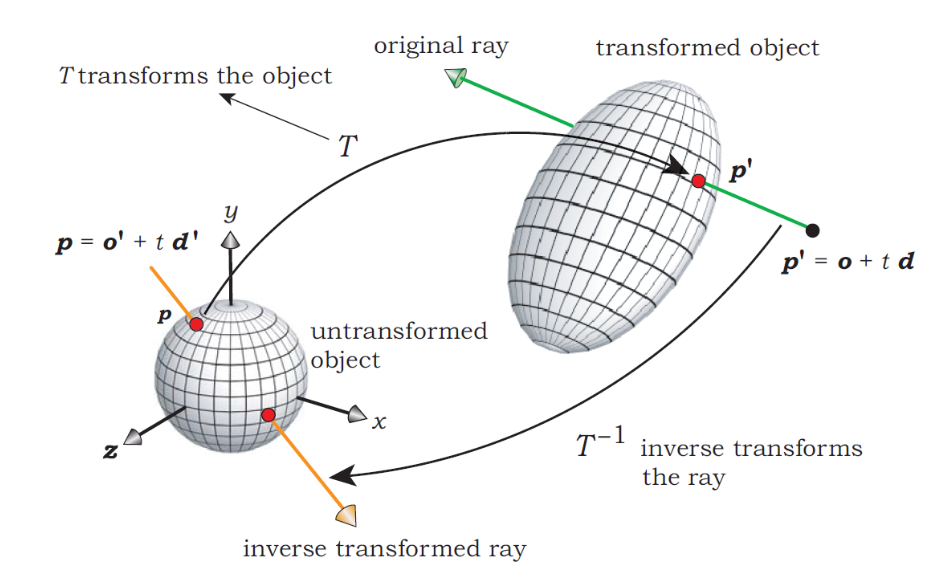
How do we intersect rays with transformed objects? We don’t! We transform the ray instead. This is done by the following steps:

• Apply the inverse set of transformations to the ray to produce the inverse transformed ray.
• Intersect the inverse transformed ray with the untransformed object.
• Compute the normal to the untransformed object at the intersection point.
• Use the intersection point on the untransformed object to compute where the original ray intersects the transformed object.
• Use the normal to the untransformed object to compute the normal to the transformed object.

A normal is always perpendicular to the surface of an object!

Simple Stochastic Ray Tracing

We can choose the number of viewing rays per pixel (anti-alising). We can also choose the number of random rays over the hemishpere for each surface point (Branching fractor).

When the branching factor is 1, we get the algorithm that is known as “Path tracing”.

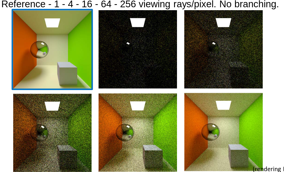
When we use 4 viewing rays per pixel, but increase the branching factor we get:

(Reference, Branching factor 1 - 2 - 4)

If we now increase the depth of the recursion, we get:

(Reference, Recursion depth 1 - 2 - 3)

How do we stop the recursion? (Russian Roulette)

Choose a ‘absorption probability’ \(\alpha\)

• Probability \(\alpha\) that a ray will not be reflected: In this case we stop the recursion
• Probability \(1 - \alpha\) that a ray will be reflected: Incoming radiance for reflected ray is multiplied by \(1/(1 - \alpha)\)

E.g. \(\alpha = 0.9\)

• \(10\%\) chance that a ray will be reflected
• If the ray is reflected, radiance along the reflected ray ‘counts’ for \(1/0.1 = 10\) times as much as radiance along the original ray

E.g. \(\alpha = 0.7\)

• \(30\%\) chance that a ray will be reflected
• If the ray is reflected, radiance along the reflected ray ‘counts’ for \(1/0.3 = 3.33333\) times as much as radiance along the original ray

E.g. \(\alpha = 0.1\)

• \(90\%\) chance that a ray will be reflected
• If the ray is reflected, radiance along the reflected ray ‘counts’ for \(1/0.9 = 1.11111\) times as much as radiance along the original ray

\(1 - \alpha\) is often set proportional to the integrated value of the BRDF

• Reflected rays are proportional to the amount of reflected light in the scene
• Computational effort is proportional to the light distribution in the 3D scene

Branching factor controls the width of the recursion tree.

Russian Roulette controls the depth of the recursion tree.