Uncertain Evidence
Table of contents
Hard Evidence
We are certain that a variable is in particular state. In this case, all the probability mass is one of the vector components. For example: \(\text{dom}(y) =\) {red, blue, green}, the vector \((0,0,1)\) represents hard evidence that \(y\) is in the state green.

Soft Evidence
In soft/uncertain evidence the variable is in more than one state, with the strength of our belief about each state being given by probabilites. For example: \(\text{dom}(y)=\) {red, blue, green}, the vector \((0.6, 0.1, 0.3)\) represents probabilities of the respective states.

Inference with soft-evidence can be achieved using Bayes’ rule. Writing the soft evidence as \(\tilde{y}\), we have:
\[p(x \mid \tilde{y}) = \sum_y p(x, y \mid \tilde{y}) = \sum_y p(x \mid y)p(y \mid \tilde{y})\]Where we make the underlying assumption:
\[p(x \mid y) = p(x\mid \tilde{y}, y)\]Example

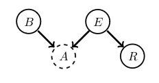
Revisiting the earthquake scenario, we think we hear a burglar alarm sounding, but are nog sure, specifically \(p(A = \text{tr}) = 0.7\). For this binary variable case we represent this soft-evidence for the states (tr, fa) as \(\tilde{A} = (0.7, 0.3)\). What is the probability of a burglary under this soft-evidence?
\[\begin{align} p(B = \text{tr} \mid \tilde{A}) &= \sum_a p(B = \text{tr}, A \mid \tilde{A}) \\ &= \sum_a p(B = \text{tr} \mid A \tilde{A})p(A \mid \tilde{A}) \\ &= \sum_a p(B = \text{tr} \mid A)p(A \mid \tilde{A}) \\ &= p(B = \text{tr} \mid A = \text{tr}) \times 0.7 + p(B = \text{tr} \mid A = \text{fa}) \times 0.3 \approx 0.6930 \end{align}\]This value is lower thatn 0.99, the probability of being burgled when we are sure we heard the alarm. The probabilites \(p(B = \text{tr} \mid A = \text{tr})\) and \(p(B = \text{tr} \mid A = \text{fa})\) are calculated using Bayes’ rule from the original distribution, as before.