Markov Network
Table of contents
Definition
A Markov Network is an undirected graph in which there is a potential (non-negative function) \(\psi\) defined on each (maximal) clique. (Maximality is not always assumed.)
The joint distribution is proportional to the product of all clique potentials:
\[p(A,B,C,D,E) = \frac{1}{Z} \psi(A,B) \psi(B,C,E) \psi(C,D)\]where \(Z\) is the normalising constant:
\[Z = \sum_{A,B,C,D,E} \psi(A,C) \psi(B,C,E) \psi(C,D)\]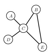
Example
Lets consider the following Markov Network:
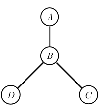
Where the factorization is:
\[p(A,B,C,D) \propto f_1(A,B) f_2(B,C) f_3(B,D)\]With the following potentials: (\(f_1\): it is 10 times more likely that A and B are in the same state than in different ones.)
| \(A\) | \(B\) | \(f_1(A,B)\) |
|---|---|---|
| 0 | 0 | 10 |
| 0 | 1 | 1 |
| 1 | 0 | 1 |
| 1 | 1 | 10 |
| \(B\) | \(C\) | \(f_2(B,C)\) |
|---|---|---|
| 0 | 0 | 1 |
| 0 | 1 | 10 |
| 1 | 0 | 10 |
| 1 | 1 | 1 |
| \(B\) | \(D\) | \(f_3(B,D)\) |
|---|---|---|
| 0 | 0 | 10 |
| 0 | 1 | 1 |
| 1 | 0 | 1 |
| 1 | 1 | 10 |
What is the most likely state?
\[p(1,1,0,1) \propto 10 \times 10 \times 10\]Ising Model
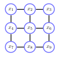
Where:
\[x_i \in \{-1,1\}:\] \[p(x_1, \dots, x_9) = \frac{1}{Z} \prod_{i \sim j} \phi_{ij}(x_i, x_j)\] \[\phi_{ij}(x_i, x_j) = e^{-\frac{1}{2T}(x_i, x_j)^2}\]\(i \sim j\) denotes the set of indices where \(i\) and \(j\) are neighbours in the graph. The potential encourages neighbours to be in the same state.
Example: Image Processing
Problem: We want to recover a binary image from the obeservation of a corrupted version of it. Where the model is defined as follows: (The white nodes are the clean pixels and the shaded nodes are the corrupted pixels.)
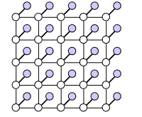
We get:
\[X = \{X_i, i=1, \dots, D\}, X_i \in \{-1,1\} \text{: clean pixel}\] \[Y = \{Y_i, i=1, \dots, D\}, Y_i \in \{-1,1\} \text{: corrupted pixel}\]A model for this situation is:
\[\phi(Y_i, X_i) = e^{\gamma X_i Y_i} \text{ encourage} X_i \text{ and } Y_i \text{ to be similar}\] \[\psi(X_i, X_j) = e^{\beta X_i X_j} \text{ encourage the image to be smooth}\] \[p(X,Y) \propto (\prod_{i=1}^D \phi(Y_i, X_i)) (\prod_{i\sim j} \psi(Y_i, X_j))\]Finding the most likely X given Y is not easy (since the graph is not singly-connected), but approximate algorithms often work well.
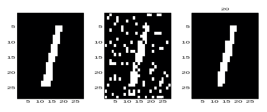
The left image is the original clean image, the middle is the observed (corruped) image and the right is the most likely clean image \(\arg\max_X p(X\mid Y)\).
Markov Properties
Factorization in Markov Models:
\[p(x_1, \dots, x_D) = \frac{1}{Z} \prod_1^C \phi_c(X_c)\]Local Markov Property - Neighbours - Markov blanket:
\[p(x \mid X \setminux x) = p(x \mid Ne(x))\]Where \(Ne(x)\) are the neighbours of \(x\) in the graph; When a distribution satisfies this property for all \(x \in X\) it is a Markov Random Field with respect to G.
Pariwise Markov Property:
\[x \!\perp\!\!\!\perp y \mid X \setminus \{x,y\}\]When \(x\) and \(y\) are not adjacent.
\[p(A,B,C) = \phi_{AC}(A,C)\phi_{BC}(B,C)\setminus(Z)\]
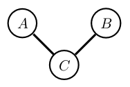
Marginalising over \(C\) makes \(A\) and \(B\) (graphically) dependent. In general \(p(A,B) \neq p(A)p(B)\).

Conditioning on \(C\) makes \(A\) and \(B\) independent: \(p(A,B \mid C) = p(A\mid C)p(B\mid C)\).

General Rule for Independence in Markov Networks
- Remove all links neighbouring the variables in the conditioning set \(Z\).
- If there is no path from any member of \(X\) to any member of \(Y\), then \(X\) and \(Y\) are conditionally independent given \(Z\).
