Learning From Fully Observed Data
Table of contents
- Learning Setting
- Scientific Inference and Learning
- Learning the bias of a coin
- Conjugate Prior
- Parameter Learning
Learning Setting
Always keep in mind whether we learn:
- The parameters of the graphical model
- Point esimation (ML, MAP)
- A distribution over these parameters (from prior to posterior)
- The Structure of the graphical model
Always keep in mind what data is available, is the data fully or partially observed?
Scientific Inference and Learning
Tell me something about the variable(s) \(\theta\) given that I have observed data \(D\) and have some knowledge of the underlying data generating mechanism:

\(p(D \mid \theta)\) are often physical models of the world which typically postulate how to generate observed phenomena, assuming we know the model.
Example: Pendulum
- \(\theta\): length, mass, damping
- \(D\): observed data of angle of pendulum over time
- \(p(D \mid \theta)\): model of probability distribution of angle over pendulum provided the parameters \(\theta\)
prior, likelihood and evidence
Learning the bias of a coin
\[v^n = \begin{cases} 1 & \text{ if on toss n the coin comes up heads} \\ 0 & \text{ if on toss n the coin comes up tails} \end{cases}\]Goal = esimate the probability that the coin will be heads
\[p(v^n = 1 \mid \theta) = \theta\]\(\theta\) is called the ‘bias’ of the coin.
Building the model
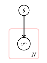
Assumptions: no dependence between the observed tosses, except trough \(\theta\): \(p(v^1, \dots, v^n, \theta) = p(\theta)\prod_{n=1}^N p(v^n \mid \theta)\)
The Likelihood
What is the likelihood of \(p(v^1, \dots, v^n \mid \theta)\)?
\[\begin{align} p(v^1, \dots, v^n \mid \theta) &= \prod_{n=1}^N p(v^n \mid \theta) \\ &= \prod_{n=1}^N \theta^{\prod[v^n=1]}(1 - \theta)^{\prod[v^n = 0]} \\ &= \theta^{\sum_{n=1}^N \prod[v^n=1]}(1 - \theta)^{\sum_{n=1}^N \prod[v^n=0]} \\ \end{align}\]Hence
\[p(v^1, \dots, v^n \mid \theta) = \theta^{N_H}(1 - \theta)^{N_T}\]\(N_H = \sum_{n=1}^N \prod[v^n=1]\) is the number of occurences of heads.
\(N_H = \sum_{n=1}^N \prod[v^n=0]\) is the number of tails.
The probability distribution over \(N_H\), the number of “successes” is the Bernoulli distribution:
\[p(v^1, \dots, v^N \mid \theta) = \theta^{N_H}(1 - \theta)^{N_T}\]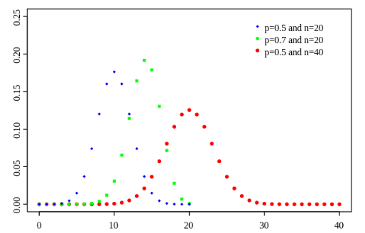
Maximum Likelihood
What is the maximum likelihood estimate of \(\theta\)?
\[\theta_{ML} = \arg \max_\theta p(v^1, \dots, v^10 \mid \theta)\] \[\theta_{ML} = \arg \max_\theta \theta^{N_H}(1 - \theta)^{N_T} = \frac{N_H}{N_H + N_T} = \frac{2}{10} = 0.2\]So the maximum likelihood is just counting the number of heads and dividing by the total number of tosses.
The Prior
What is the prior distribution over \(\theta\)?
Assume a discrete prior:
\[p(\theta = 1) = 0.15, p(\theta = 0.5) = 0.8, p(\theta = 0.8) = 0.05\]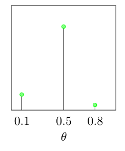
The Posterior
Do the actual calculations of the posterior for the prior:
\[p(\theta = 1) = 0.15, p(\theta = 0.5) = 0.8, p(\theta = 0.8) = 0.05\]And the observations: 1, 0, 0, 0, 0, 0, 1, 0, 0, 0
Remember: \(p(\theta \mid v^1, \dots, v^N) \propto p(\theta)\theta^{N_H}(1 - \theta)^{N_T}\) so: \(N_H = 2, N_T = 8\) And: As the prior distribution is discrete with possible states 0.1, 0.5, and 0.8; the posterior distribution will also be discrete limited to the states.
\[\begin{align} p(\theta = 0.1 \mid v^1, \dots, v^N) &\propto 0.15 \times 0.1^2(1-0.1)^8) \\ p(\theta = 0.5 \mid v^1, \dots, v^N) &\propto 0.8 \times 0.5^2(1-0.5)^8) \\ p(\theta = 0.8 \mid v^1, \dots, v^N) &\propto 0.05 \times 0.8^2(1-0.8)^8) \\ \end{align}\]After normalization the posterior is obtained:
\[\begin{align} p(\theta = 0.1 \mid v^1, \dots, v^N) &= 0.452 \\ p(\theta = 0.5 \mid v^1, \dots, v^N) &= 0.547 \\ p(\theta = 0.8 \mid v^1, \dots, v^N) &= 0.001 \\ \end{align}\]Graphically we get:
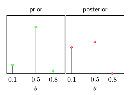
So we get:
\[\text{ML-esimtae}: \theta_* = 0.2\] \[\text{MAP-esimtae}: \theta_* = 0.5\]Continuous Distributions
What if \(\theta\) is not limited discrete but continuous?
Prior: \(\theta \in [0,1]\): flat prior \(p(\theta) = 1\)
Posterior: \(p(\theta \mid V) = \frac{1}{c} \theta^{N_H}(1 - \theta)^{N_T}\), with \(c\) the normalization constant.
\(c= \int_0^1 \theta^{N_H}(1 - \theta)^{N_T} d\theta = B(N_H + 1, N_T + 1)\) with \(B(\alpha, \beta)\) the Beta function.
Conjugate Prior
The conjugate prior is the prior such that the posterior is of the same family of probability distributions.
Coin tossing case
If prior is the beta distribution:
\[p(\theta) = B(\theta \mid \alpha, \beta) = \frac{1}{B(\alpha, \beta)} \theta^{\alpha - 1}(1 - \theta)^{\beta - 1}\]Then the posterior is also a beta distribution:
\[\begin{align} p(\theta \mid V) &\propto \theta^{\alpha - 1}(1 - \theta)^{\beta - 1} \theta^{N_H}(1 - \theta)^{N_T} \\ &= \frac{1}{B(\alpha + N_H, \beta + N_T)} \theta^{\alpha + N_H - 1}(1 - \theta)^{\beta + N_T - 1} \\ &= B(\theta \mid \alpha + N_H, \beta + N_T) \end{align}\]Beta distribution is the ‘conjugate’ to the Binomial distribution.
\(\alpha\) and \(\beta\) sometimes are called “virtual counts”.
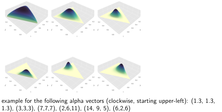
There are two distributions we can use for conjugate priors:
- Beta distribution for binary attributes (heads or tails)
- Dirichlet distribution for multi-valued attributes
Parameter Learning
Consider the following model of the relationship between exposure to asbestos (a), being a smoker (s) and the probability of getting lung cancer (c):
\[p(a,s,c) = p(c \mid a,s)p(a)p(s)\]Each variable is binary. Furthermore, we assume that we have a list of patients, where each row represents a patient’s data.
| a | s | c |
|---|---|---|
| 1 | 1 | 1 |
| 1 | 0 | 0 |
| 0 | 1 | 1 |
| 0 | 1 | 0 |
| 1 | 1 | 1 |
| 0 | 0 | 0 |
| 1 | 0 | 1 |
The ML is just counting the number of times a certain combination of values occurs and dividing by the total number of patients.
To learn the table entries \(p(c \mid a,s)\) we can dos so by counting the number of \(c\) is in state 1 for each of the 4 parental states of \(a\) and \(s\):
\[p(c = 1 \mid a = 0, s = 0) = 0\] \[p(c = 1 \mid a = 1, s = 0) = 0.5\] \[p(c = 1 \mid a = 0, s = 1) = 0.5\] \[p(c = 1 \mid a = 1, s = 1) = 1\]Similarly, based on counting \(p(a = 1) = 4/7\), and \(p(s = 1) = 4/7\). These three CPTs then complete the full distribution specification.
Kullback-Leibler Divergence
\[KL(q\mid p) = \langle \log q(x) - \log p(x) \rangle_{q(x)} \geq 0\]Where:
- \(\langle f(x) \rangle_{r(x)}\) denotes the expected value of \(f(x)\) w.r.t. the distribution \(r(x)\)
- \(\langle f(x) \rangle_{r(x)} = \int f(x) r(x) dx\) in continuous cases
- \(\langle f(x) \rangle_{r(x)} = \sum_x f(x) r(x)\) in discrete cases
- KL divergence is 0 iff the two distributions are exactly the same
- KL divergence measures the difference of the distributions \(p\) and \(q\)
- KL divergence is not symmetric, in generel \(KL(q \mid p) \neq KL(p \mid q)\)
Maximizing the likelihood corresponds to minimizing the KL-divergence between the “empirical data distribution” (what the data shows \(q(x) = p_D(x)\)) and the modeled distribution \(p(x \mid \theta)\)
ML for Naive Bayes
Consider the following vector of attributes: (likes shortbread, likes lager, drinks whiskey, eats porridge, watched England play football)
Together with each vector \(x\), there is a label \(nat\) describing the nationality of the person, \(dom(nat) = \{English, Scottish\}\).
We can use Bayes’ rule to calculate the probability that \(x\) is Scottish or English:
\[\begin{align}p(\text{Scottish} \mid x) &= \frac{p(x \mid \text{Scottish})p(\text{Scottish})}{p(x)} \\ &= \frac{p(x \mid \text{Scottish})p(\text{Scottish})}{p(x \mid \text{Scottish})p(\text{Scottish}) + p(x \mid \text{English})p(\text{English})}\end{align}\]For \(p(x \mid nat)\) under the Naive Bayes assumption we can write:
\[p(x \mid nat) = \prod_{i=1}^5 p(x_i \mid nat)\]Lets say we have the following data:

Using Maximum Likelihood we have: \(p(\text{Scottish}) = 7/13\) and \(p(\text{English}) = 6/13\) (we have 13 data points in total, of which 7 are Scottish and 6 are English).
\[p(x_1 = 1 \mid \text{English}) = 1/2 \quad p(x_1 = 1 \mid \text{Scottish}) = 1\] \[p(x_2 = 1 \mid \text{English}) = 1/2 \quad p(x_2 = 1 \mid \text{Scottish}) = 4/7\] \[p(x_3 = 1 \mid \text{English}) = 1/3 \quad p(x_3 = 1 \mid \text{Scottish}) = 3/7\] \[p(x_4 = 1 \mid \text{English}) = 1/2 \quad p(x_4 = 1 \mid \text{Scottish}) = 5/7\] \[p(x_5 = 1 \mid \text{English}) = 1/2 \quad p(x_5 = 1 \mid \text{Scottish}) = 3/7\]For \(x = (1,0,1,1)^T\), we get:
\[p(\text{scottish} \mid x) = \frac{1 \times \frac{3}{7} \times \frac{3}{7} \times \frac{5}{7} \times \frac{4}{7} \times \frac{7}{13}}{1 \times \frac{3}{7} \times \frac{3}{7} \times \frac{5}{7} \times \frac{4}{7} \times \frac{7}{13} + \frac{1}{2} \times \frac{1}{2} \times \frac{1}{3} \times \frac{1}{2} \times \frac{1}{2} \times \frac{6}{13}} = 0.8076\]Since this is greater than 0.5, we would classify this person as Scottish.
Notes:
- When we have sparse data, it will result in 0 or 1 entries in the table for ML, this is unlikely (overfitting), avoid is by using a Bayesian approach (using a prior).
- Multi-valued values: do not formulate as \(n\) binary attributes, this violates the conditional independence assumptions
- It is frequently used in spam-filtering, text classification, etc.
- It is a efficient and simple method, but it is not very accurate
MAP
We continue with the Asbestos, Smoking and Cancer example.
\[p(a,c,s) = p(c \mid a,s)p(a)p(s)\]and a set of visible observations \(V = \{(a^n, s^n, c^n)\, n = 1, \dots, N\}\). With all variables binary, we have parameters such as:
\[p(a = 1 \mid \theta_a) = \theta_a, \quad p(c=1 \mid a=0,s=1, \theta_c) = \theta_c^{0,1}\]The parameters are:
\[\theta_a, \theta_s, \theta_c^{0,0}, \theta_c^{0,1}, \theta_c^{1,0}, \theta_c^{1,1}\]\(\theta_c^{0,0}\) is the probability of cancer when \(a = 0\) and \(s = 0\).
\[p(\theta_c) = p(\theta_c^{0,0}) p(\theta_c^{0,1}) p(\theta_c^{1,0}) p(\theta_c^{1,1})\]Beta Prior
\[p(a = 1 \mid V_a) = E[\theta_a] = \frac{\alpha_a + \#(a=1)}{\alpha_a + \#(a=1) + \beta_a + \#(a=0)}\]The prior parameters \(\alpha_a, \beta_a\) are called hyperparameters. If one had no preference, one would set \(\alpha_a = \beta_a = 1\).
